CABEAN: A Software Tool for the Control of Asynchronous Boolean Networks

Description

CABEAN is a software tool for the control of asynchronous Boolean networks, which are often used to model gene regulatory networks.

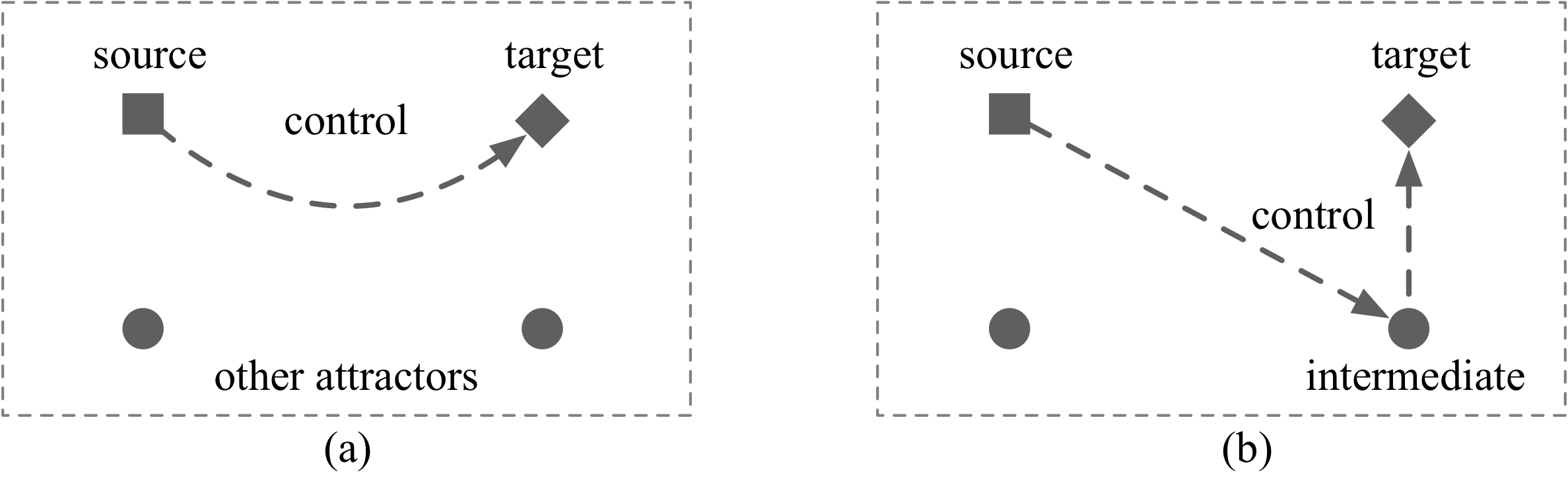
The source-target control of asynchronous Boolean networks can be achieved either in one step, called one-step control, or in multiple steps, called sequential control. Taking difficulties in practical applications into consideration, we are particularly interested in the sequential control through other attractors, called attractor-based sequential control. Figure 1(a) and Figure 1(b) illustrate the one-step and attractor-based sequential control, respectively. Squares and rhombuses represent the source and target attractors. Circles represent the other attractors of the network. One-step control drives the network from the source directly to the target, while attractor-based sequential control employs other attractors as intermediate and identifies a sequence of perturbations. Based on the application time of control, we have instantaneous, temporary and permanent controls. Instantaneous control applies perturbations instantaneously; temporary control applies perturbations for sufficient time and then released; and permanent control applies the control for all the following time steps.

Figure 1. (a) One-step and (b) attractor-based sequential source-target control of Boolean networks.

Combining the two categories, there are six different control strategies. CABEAN provides the following methods to solve the six source-target control problems:

the minimal one-step instantaneous source-target control (OI) [BCB18, TCBB19];
the minimal one-step temporary source-target control (OT) [FM19];
the minimal one-step permanent source-target control (OP) [FM19];
attractor-based sequential instantaneous source-target control (ASI) [CMSB19];
attractor-based sequential temporary source-target control (AST) [CMSB20];
attractor-based sequential permanent source-target control (ASP) [CMSB20].

CABEAN provides the following target control methods:

instantaneous target control (ITC) [BCB20];
temporary target control (TTC) [BCB20];
permanent target control (PTC).

Download

CABEAN is freely available. The newest version of CABEAN is 2.0.1, updated on May 10, 2021. You can download the files here, including executable binaries for Windows, Mac or Linux, a detailed user guide and examples. Starting from version 1.0.1, CABEAN supports model files under BoolNet format.

Version 1.0.0 updated on April 17, 2020.
Version 1.0.2 updated on July 14, 2020.
Version 2.0.0 updated on October 26, 2020.

Requirements

1. Platform: x86 compatible 32 bit or 64 bit processor;

2. Operating system: Windows, Linux and Mac OSX (10.4 and above);

3. Required compilers: flex 2.6.4 or higher, GNU bison 3.0.4 or higher, GNU g++ 4.0.1 or higher, and Windows subsystem for Linux (Windows platform only).

Quickstart Guide

In this quick guide, we use two examples to illustrate the basic usages of CABEAN, including the syntax of the model file and how to compute different controls with and without practical constraints. Specifically, Example 1 focuses on the introduction of different control methods and Example 2 shows how to encode practical constraints. For detailed introduction of CABEAN, please download the user guide.

Example 1

How to define a Boolean network?

Nodes Functions Indices of attractors Attractors

x₁ f₁= x₂ A₁ 000

x₂ f₂= x₁ A₂ 110

x₃ f₃= x₂ ∧ x₃ A₃ 111

Nodes	Functions	Indices of attractors	Attractors
x₁	f₁= x₂	A₁	000
x₂	f₂= x₁	A₂	110
x₃	f₃= x₂ ∧ x₃	A₃	111

Table 1. The Boolean functions and the attractors of Example 1.

The first two columns of Table 1 describe a Boolean network with three nodes, including x₁, x₂, x₃. Each node is assigned with a Boolean function. CABEAN supports the BoolNet and ISPL (Interpreted Systems Programming Language) format. We recommend the BioLQM toolkits for the conversion of other formats, such as SBML-qual, Petri net, GINsim, to BoolNet format. BioLQM is available at http://colomoto.org/biolqm/.
BoolNet describes a Boolean network or probabilistic Boolean network in a standardized text file format. Here we only explain the syntax for Boolean networks. The model file of the example under BoolNet format is given below. The first line is a header: 'targets, factors'. The name and the Boolean function of each node are separated by a comma and given at each line. The header implies the format: 'targets' is the name of the node and 'factors' represents the Boolean function of the node. In the Boolean functions, the logical operators 'and', 'or' and 'not' are represented as '&', '|' and '!'. Users can initialise the value of an input node to either '1' or '0'.

  targets, factors
  x1, x2
  x2, x1
  x3, x2&x3

The model file of Example 1 under BoolNet format. (Download: toy.bnet)

The model file under ISPL format is shown below. It contains two sections: section 'Agent M' and section 'InitStates'. Section 'Agent M' defines the Boolean variables and the Boolean functions of the network; section 'InitStates' specifies the initial state. Section 'Agent M' includes four parts: 'Vars', 'Actions', 'Protocol', and 'Evolution'. The 'Vars' part defines the Boolean variables and the order of the variables is consistent with the order of the nodes in each state in the output. The 'Evolution' part specifies the Boolean functions for each variable. The functions are defined using parenthesis and three logical operations, including logical and '&', logical or '|', and logical not '~'. The 'Actions' and 'Protocol' parts are defined as '{none}'. The ISPL format is preferable than BoolNet format. In the following sections, we use 'toy.ispl' as the name of the model file.

  Agent M
    Vars:    
      x1: boolean;
      x2: boolean;    
      x3: boolean;
    end Vars
    Actions = {none};
    Protocol:
      Other: {none};
    end Protocol
    Evolution:
      x1=true  if  x2=true;
      x1=false if  x2=false;    
      x2=true  if  x1=true;
      x2=false if  x1=false;
      x3=true  if  x2&x3=true;
      x3=false if  x2&x3=false;
    end Evolution
  end Agent

  InitStates
      M.x1=true or M.x1=false;
  end InitStates

The model file of Example 1 under ISPL format. (Download: toy.ispl)

Figure 2. (a) The original ransition system (b) transition system under control C₁={x2=1 x3=1} and (c) transition system under control C₂={x1=1 x3=1} of Example 1. We omit self-loops for all the states except for state (101) in (a).

How to compute the attractors of the network?

CABEAN implements the decomposition-based attractor detection method [APBC18] that can identify all the exact attractors of the network. The attractors of the example can be computed using the following command:

./cabean -compositional 2 toy.ispl

The output of CABEAN is given below. This network has three attractors. In each state, the sequence of the nodes is consistent with the sequence of the nodes defined in the model file. The transition system of the network under asynchronous updating scheme is given in Figure 2(a). We can see that the attractors #1, #2 and #3 identified by our methods correspond to A₁, A₂ and A₃ in Figure 2(a). From any initial state, the network will eventually settle down to one of the attractors.

Command line: ./cabean -compositional 2 toy.ispl
======================== find attractor #1 : 1 states ========================
: 4 nodes 1 leaves 1 minterms
0-0-0-  1

======================== find attractor #2 : 1 states ========================
: 4 nodes 1 leaves 1 minterms
1-1-0-  1

======================== find attractor #3 : 1 states ========================
: 4 nodes 1 leaves 1 minterms
1-1-1-  1

number of attractors = 3
time for attractor detection=0.001 seconds

Attractors of Example 1. (Download: toy-attractors.txt)

How to compute the control for one pair of source and target attractors?

In the previous section, we showed how to use CABEAN for the identification of attractors. Below is a template command line for computing the control from the source attractor to the target attractor.

./cabean -compositional 2 -control <control method> -sin <indice of the source> -tin <indice of the target> <model file>

In the command line, '-compositional 2' implies that the strong basin of an attractors is computed using the decomposition-based computation methods [BCB18, TCBB19]; '-control <control method>' indicates the control method (OI, OT, OP, ASI, AST or ASP); '-sin <indice of the source> -tin <indice of the target>' indicates the indices of the source and target attractors; '<model file>' is the path of the model file and it is always placed at the end of the command line. In this way, the source and target correspond to one of the attractors of the network. The attractor can be either a single-state attractor or a cyclic attractor. If the source attractor is cyclic, CABEAN will identify the control to be applied to a state in the source attractor that requires the fewest number of perturbations. Currently, CABEAN does not support the control from/to a set of attractors.
CABEAN first identifies all the exact attractors of the network and then compute the control for the specified source and target attractors. For this example, let us assume A₁ and A₃ are the source and the target attractors, respectively. Next we show how to compute OI, OT, OP, ASI, AST and ASP from A₁ to A₃ with CABEAN.

Minimal OI control

We use the following command line to compute the minimal OI control from A₁ to A₃ for Example 1.

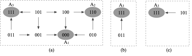
./cabean -compositional 2 -control OI -sin 1 -tin 3 toy.ispl

The results are shown below. CABEAN identifies one minimal OI control {x1=1 x2=1 x3=1}. To compute the minimal OI contol, our method computes the strong basin of the target attractor and then finds the intermediate state in the strong basin that has the shortest Hamming distance to the source state. The nodes that have different values in the source state and the intermediate state are the driver nodes. Figure 2(a) shows that the strong basin of A₃ contains only one state (111). Thus, the minimal OI control drives the network from (000) to (111) and the associate control set is {x1=1 x2=1 x3=1}.

Command line: ./cabean -compositional 2 -control OI -sin 1 -tin 3 toy.ispl
======================== find attractor #1 : 1 states ========================
: 4 nodes 1 leaves 1 minterms
0-0-0-  1

======================== find attractor #2 : 1 states ========================
: 4 nodes 1 leaves 1 minterms
1-1-0-  1

======================== find attractor #3 : 1 states ========================
: 4 nodes 1 leaves 1 minterms
1-1-1-  1

number of attractors = 3
time for attractor detection=0.001 seconds

====== ONE-STEP INSTANTANEOUS SOURCE-TARGET CONTROL (DECOMP) ======

source - 1 target - 3

PATH 1 - #perturbations: 3
  Control set: x1=1 x2=1 x3=1 
execution time of control  = 0 seconds

Results of the minimal OI control of Example 1 from A₁ to A₃. (Download: toy-OI.txt)

Minimal OT control

We use the following command line to compute the minimal OT control from A₁ to A₃ for Example 1.

./cabean -compositional 2 -control OT -sin 1 -tin 3 toy.ispl

The results are shown below. To compute the minimal OT contol, our method explores the weak basin of the target attractor starting from the state that has the shortest Hamming distance to the source state and verify if the corresponding control is a valid temporary control or not. If so, we are done and the control is the minimal OT control. Otherwise, we proceed to the next state that has the shortest Hamming distance to the source state and repeat the verification process. As shown in Figure 2(a), the weak basin of A₃ consists of three states: (011), (101) and (111). States (011) and (101) have the shortest Hamming distance to A₁. For state (011), the corresponding control set is C₁={x2=1 x3=1}. The application control of C₁ stirs the network from state (000) to (011) and reshapes the transition system from Figure 2(a) to Figure 2(b). During the control, the network will eventually and surely reach the target attractor A₃. Therefore, C₁ is a minimal OT control. Similarly, we can prove that the control C₂={x1=1 x3=1} associated with the intermediate state (011) is also a minimal OT control. (Figure 2(c) shows the transition system under control C₂. )

Command line: ./cabean -compositional 2 -control OT -sin 1 -tin 3 toy.ispl
======================== find attractor #1 : 1 states ========================
: 4 nodes 1 leaves 1 minterms
0-0-0-  1

======================== find attractor #2 : 1 states ========================
: 4 nodes 1 leaves 1 minterms
1-1-0-  1

======================== find attractor #3 : 1 states ========================
: 4 nodes 1 leaves 1 minterms
1-1-1-  1

number of attractors = 3
time for attractor detection=0 seconds

====== ONE-STEP TEMPORARY SOURCE-TARGET CONTROL (DECOMP) ======

source - 1 target - 3

PATH 1 - #perturbations: 2
  Control set: x2=1 x3=1 

PATH 2 - #perturbations: 2
  Control set: x1=1 x3=1 
execution time for control = 0.001 seconds

Results of the minimal OT control of Example 1 from A₁ to A₃. (Download: toy-OT.txt)

Minimal OP control

We use the following command line to compute the minimal OP control from A₁ to A₃ for Example 1. The results of the minimal OP control are the same with the minimal OT control. To avoid duplication, we omit the output of OP control here (toy-OP.txt).

./cabean -compositional 2 -control OP -sin 1 -tin 3 toy.ispl

ASI control

We use the following command line to compute the minimal ASI control from A₁ to A₃ for Example 1.

./cabean -compositional 2 -control ASI -sin 1 -tin 3 toy.ispl

ASI control identifies a sequence of instantaneous perturbations to drive the dynamics from the source to the target passing through other attractors In the current implementation, the number of perturbations required by the minimal OI control is adopted as the threshold on the number of perturbations. We have shown that the minimal OI control from A₁ to A₃ requires at least three perturbatons. ASI identifies one sequential control path with three perturbations as shown below. It first flips the values of node x1 and x2 from 0 to 1, which drives the network from A₁ to the intermediate attractor A₂. Then it flips the value of x3, which leads the network from A₂ to A₃.

Command line: ./cabean -compositional 2 -control ASI -sin 1 -tin 3 toy.ispl
======================== find attractor #1 : 1 states ========================
: 4 nodes 1 leaves 1 minterms
0-0-0-  1

======================== find attractor #2 : 1 states ========================
: 4 nodes 1 leaves 1 minterms
1-1-0-  1

======================== find attractor #3 : 1 states ========================
: 4 nodes 1 leaves 1 minterms
1-1-1-  1

number of attractors = 3
time for attractor detection=0.001 seconds

========= ATTRACTOR-BASED SEQUENTIAL INSTANTANEOUS SOURCE-TARGET CONTROL (DECOMP) =========

source - 1 target - 3

PATH 1 - #perturbations: 3
Sequence of the attractors: 1 -> 3
  STEP 1
    Control set 1: x1=1 x2=1 x3=1 

PATH 2 - #perturbations: 3
Sequence of the attractors: 1 -> 2 -> 3
  STEP 1
    Control set 1: x1=1 x2=1 
  STEP 2
    Control set 1: x3=1 
execution time of control=0 seconds

Results of ASI control of Example 1 from A₁ to A₃. (Download: toy-ASI.txt)

AST control

We use the following command to compute the minimal AST control from A₁ to A₃ for Example 1.

./cabean -compositional 2 -control AST -sin 1 -tin 3 toy.ispl

AST control identifies a sequence of temporary perturbations to drive the dynamics from the source to the target passing through other attractors of the network. In the current implementation, the number of perturbations required by the minimal OT control is adopted as the threshold for AST. For this example, AST identifies two sequential control paths with two perturbations as shown below. Similar to ASI control, AST control also employs A₂ as the intermediate attractor. There exist two temporary control sets from A₁ to A₂: {x1=1} and {x2=1}. The control set from A₂ to A₃ is the same as that of ASI control.

Command line: ./cabean -compositional 2 -control AST -sin 1 -tin 3 toy.ispl
======================== find attractor #1 : 1 states ========================
: 4 nodes 1 leaves 1 minterms
0-0-0-  1

======================== find attractor #2 : 1 states ========================
: 4 nodes 1 leaves 1 minterms
1-1-0-  1

======================== find attractor #3 : 1 states ========================
: 4 nodes 1 leaves 1 minterms
1-1-1-  1

number of attractors = 3
time for attractor detection=0 seconds

========= ATTRACTOR-BASED SEQUENTIAL TEMPORARY SOURCE-TARGET CONTROL (DECOMP) =========

source - 1 target - 3

PATH 1 - #perturbations: 2
Sequence of the attractors: 1 -> 3
  STEP 1
    Control set 1: x2=1 x3=1 
    Control set 2: x1=1 x3=1 

PATH 2 - #perturbations: 2
Sequence of the attractors: 1 -> 2 -> 3
  STEP 1
    Control set 1: x2=1 
    Control set 2: x1=1 
  STEP 2
    Control set 1: x3=1 
execution time of control=0.002 seconds

Results of AST control of Example 1 from A₁ to A₃. (Download: toy-AST.txt)

ASP control

We use the following command to compute the minimal ASP control from A₁ to A₃ for Example 1. The results of ASP control are the same with AST control. To avoid duplication, we omit the output of ASP control here (toy-ASP.txt).

./cabean -compositional 2 -control ASP -sin 1 -tin 3 toy.ispl

How to compute the target control?

TTC

We use the following command to compute TTC to A₃ for Example 1.

./cabean -compositional 2 -control TTC -tin 3 toy.ispl

Command line: ./cabean -compositional 2 -control TTC -tin 3 toy.ispl
======================== find attractor #1 : 1 states ========================
: 4 nodes 1 leaves 1 minterms
0-0-0-  1

======================== find attractor #2 : 1 states ========================
: 4 nodes 1 leaves 1 minterms
1-1-0-  1

======================== find attractor #3 : 1 states ========================
: 4 nodes 1 leaves 1 minterms
1-1-1-  1

number of attractors = 3
time for attractor detection=0.002 seconds

=================== TEMPORARY TARGET COTNROL (DECOMP) ===================

************************************************************
TARGET ATTRACTOR #3
************************************************************

Control set 1: x1=1 x3=1 
Control set 2: x2=1 x3=1 

Time for temporary target control = 0.001 seconds

Results of TTC of Example 1 to A₃. (Download: toy-TTC.txt)

Example 2

Model files

Nodes Functions Indices of attractors Attractors

x₁ f₁= x₂ A₁ 001100

x₂ f₂= x₁ A₂ 001111

x₃ f₃= (~x₂) ∨ x₄ A₃ 110000

x₄ f₄= x₃ A₄ 110010

x₅ f₅= (x₁ ∨ x₆) ∧ x₅ A₅ 111100

x₆ f₆=x₄ ∧ x₅ A₆ 111111

Nodes	Functions	Indices of attractors	Attractors
x₁	f₁= x₂	A₁	001100
x₂	f₂= x₁	A₂	001111
x₃	f₃= (~x₂) ∨ x₄	A₃	110000
x₄	f₄= x₃	A₄	110010
x₅	f₅= (x₁ ∨ x₆) ∧ x₅	A₅	111100
x₆	f₆=x₄ ∧ x₅	A₆	111111

Table 2. The Boolean functions and the attractors of Example 2.

The first two columns of Table 2 describe a Boolean network with six nodes, including x₁, x₂, x₃, x₄, x₅, and x₆. The model file under BoolNet format is given below.

  targets, factors
  x1, x2
  x2, x1
  x3, (!x2)|x4
  x4, x3
  x5, (x1|x6)&x5
  x6, x4&x5

The model file of Example 2 under BoolNet format. (Download: example.bnet)

The model file under ISPL format is shown below.

  Agent M
    Vars:    
      x1: boolean;
      x2: boolean;    
      x3: boolean;
      x4: boolean;
      x5: boolean;
      x6: boolean;
    end Vars
    Actions = {none};
    Protocol:
      Other: {none};
    end Protocol
    Evolution:
      x1=true  if  x2=true;
      x1=false if  x2=false;    
      x2=true  if  x1=true;
      x2=false if  x1=false;
      x3=true  if  (~x2)|x4=true;
      x3=false if  (~x2)|x4=false;
      x4=true  if  x3=true;
      x4=false if  x3=false;
      x5=true  if  (x1|x6)&x5=true;
      x5=false if  (x1|x6)&x5=false;
      x6=true  if x4&x5=true;
      x6=false if x4&x5=false;
    end Evolution
  end Agent

  InitStates
      M.x1=true or M.x1=false;
  end InitStates

The model file of Example 2 under ISPL format. (Download: example.ispl)

Attractors

The attractors of Example 2 can be computed using the following command:

./cabean -compositional 2 example.ispl

The output of CABEAN is given below. This network has six attractors. Once the attractors are computed, users can use the provided functions to compute the minimal control for one pair of source and target attractors or for all combinations of source and target attractors.

Command line: ./cabean -compositional 2 example.ispl
======================== find attractor #1 : 1 states ========================
: 7 nodes 1 leaves 1 minterms
0-0-1-1-0-0-  1

======================== find attractor #2 : 1 states ========================
: 7 nodes 1 leaves 1 minterms
0-0-1-1-1-1-  1

======================== find attractor #3 : 1 states ========================
: 7 nodes 1 leaves 1 minterms
1-1-0-0-0-0-  1

======================== find attractor #4 : 1 states ========================
: 7 nodes 1 leaves 1 minterms
1-1-0-0-1-0-  1

======================== find attractor #5 : 1 states ========================
: 7 nodes 1 leaves 1 minterms
1-1-1-1-0-0-  1

======================== find attractor #6 : 1 states ========================
: 7 nodes 1 leaves 1 minterms
1-1-1-1-1-1-  1

number of attractors = 6
time for attractor detection=0.003 seconds

Attractors of the Example 2. (Download: example-attractors.txt)

How to compute the control for one pair of source and target attractors with constraints on perturbations?

We use the minimal OT control from A₆ to A₁ of Example 2 as an example to show how to compute the control for one pair of source and target attractors with constraints on perturbations. We first give the results of the minimal OT control without constraints below. We can see that CABEAN identifies eight minimal OT control sets and each control requires two perturbations.

Command line: ./cabean -compositional 2 -control OT -sin 6 -tin 1 example.ispl
======================== find attractor #1 : 1 states ========================
: 7 nodes 1 leaves 1 minterms
0-0-1-1-0-0-  1

======================== find attractor #2 : 1 states ========================
: 7 nodes 1 leaves 1 minterms
0-0-1-1-1-1-  1

======================== find attractor #3 : 1 states ========================
: 7 nodes 1 leaves 1 minterms
1-1-0-0-0-0-  1

======================== find attractor #4 : 1 states ========================
: 7 nodes 1 leaves 1 minterms
1-1-0-0-1-0-  1

======================== find attractor #5 : 1 states ========================
: 7 nodes 1 leaves 1 minterms
1-1-1-1-0-0-  1

======================== find attractor #6 : 1 states ========================
: 7 nodes 1 leaves 1 minterms
1-1-1-1-1-1-  1

number of attractors = 6
time for attractor detection=0.001 seconds

====== ONE-STEP TEMPORARY SOURCE-TARGET CONTROL (DECOMP) ======

source - 6 target - 1

PATH 1 - #perturbations: 2
  Control set: x2=0 x6=0 

PATH 2 - #perturbations: 2
  Control set: x2=0 x5=0 

PATH 3 - #perturbations: 2
  Control set: x2=0 x4=0 

PATH 4 - #perturbations: 2
  Control set: x2=0 x3=0 

PATH 5 - #perturbations: 2
  Control set: x1=0 x6=0 

PATH 6 - #perturbations: 2
  Control set: x1=0 x5=0 

PATH 7 - #perturbations: 2
  Control set: x1=0 x4=0 

PATH 8 - #perturbations: 2
  Control set: x1=0 x3=0 
execution time for control = 0.003 seconds

Results of the minimal OT control of Example 2 from A₆ to A₁. (Download: example-OT-6to1.txt)

CABEAN allows users to specify undesired perturbations and compute the minimal control excluding those perturbations. In the current version, user can define three types of perturbaions:

R0: the nodes that can not be perturbed from 0 to 1;
R1: the nodes that can not be perturbed from 1 to 0;
R: the nodes that can not be perturbed in either way.

Suppose node x₅ can not be flipped from 1 to 0 and nodes x₄ and x₆ can not be perturbed in any direction. The specification file is given below.

R0: 
R1: x5
R: x4, x6

File for the specification of undesired perturbations. (Download: rmPert.txt)

To compute the minimal OT control from A₆ to A₁ without undesired perturbations, we add the option '-rmPert <file name>' to the command line as follows:

./cabean -compositional 2 -control OT -sin 6 -tin 1 -rmPert rmPert.txt example.ispl

The output of CABEAN is given below. We can see that the minimal OT control still requires at least two perturbations and there are two solutions without undesired perturbations.

Command line: ./cabean -compositional 2 -control OT -sin 6 -tin 1 -rmPert rmPert.txt example.ispl
======================== find attractor #1 : 1 states ========================
: 7 nodes 1 leaves 1 minterms
0-0-1-1-0-0-  1

======================== find attractor #2 : 1 states ========================
: 7 nodes 1 leaves 1 minterms
0-0-1-1-1-1-  1

======================== find attractor #3 : 1 states ========================
: 7 nodes 1 leaves 1 minterms
1-1-0-0-0-0-  1

======================== find attractor #4 : 1 states ========================
: 7 nodes 1 leaves 1 minterms
1-1-0-0-1-0-  1

======================== find attractor #5 : 1 states ========================
: 7 nodes 1 leaves 1 minterms
1-1-1-1-0-0-  1

======================== find attractor #6 : 1 states ========================
: 7 nodes 1 leaves 1 minterms
1-1-1-1-1-1-  1

number of attractors = 6
time for attractor detection=0.002 seconds

====== ONE-STEP TEMPORARY SOURCE-TARGET CONTROL (DECOMP) ======

source - 6 target - 1

PATH 1 - #perturbations: 2
  Control set: x2=0 x3=0 

PATH 2 - #perturbations: 2
  Control set: x1=0 x3=0 
execution time for control = 0.001 seconds

Results of the minimal OT control of Example 2 from A₆ to A₁ with constraints on perturbations. (Download: example-OT-6to1-rmPert.txt)

How to compute the control for all pairs of source and target attractors?

CABEAN allows users to compute the control for all combinations of source and target attractors by replacing '-sin <indice of the source> -tin <indice of the target>' with '-allpairs' in the command line. The minimal OT control for all pairs of source and target attractors of the example can be computed using the following command line:

./cabean -compositional 2 -control OT -allpairs example.ispl

The results can be downloaded here (example-OT-allpairs.txt).

How to compute attractor-based sequential control with constraints on the intermediate attractors?

For attractor-based sequential control (ASI, AST and ASP), undesired attractors, such as attractors that correspond to diseased cells, can be avoided from being adopted as intermediate attractors. Suppose attractors A₂ and A₅ are the undesired ones, we can define them in the file 'rmID.txt' as follows (the indices are separated by comma):

2,5

File for the speicification of undesired attractors. (Download: rmID.txt)

Taking ASI control as an example, we first show the results without any predefined constraints below. Note that ASI control use the minimal number of perturations required by the minimal OI control as the threshold and computes all the sequential paths within the threshold. We can see that besides the one-step control paths, there are two sequential control paths from A₆ to A₁, where A₂ and A₅ act as the intermediate attractors, respectively.

Command line: ./cabean -compositional 2 -control ASI -sin 6 -tin 1 example.ispl
======================== find attractor #1 : 1 states ========================
: 7 nodes 1 leaves 1 minterms
0-0-1-1-0-0-  1

======================== find attractor #2 : 1 states ========================
: 7 nodes 1 leaves 1 minterms
0-0-1-1-1-1-  1

======================== find attractor #3 : 1 states ========================
: 7 nodes 1 leaves 1 minterms
1-1-0-0-0-0-  1

======================== find attractor #4 : 1 states ========================
: 7 nodes 1 leaves 1 minterms
1-1-0-0-1-0-  1

======================== find attractor #5 : 1 states ========================
: 7 nodes 1 leaves 1 minterms
1-1-1-1-0-0-  1

======================== find attractor #6 : 1 states ========================
: 7 nodes 1 leaves 1 minterms
1-1-1-1-1-1-  1

number of attractors = 6
time for attractor detection=0.002 seconds

========= ATTRACTOR-BASED SEQUENTIAL INSTANTANEOUS SOURCE-TARGET CONTROL (DECOMP) =========

source - 6 target - 1

PATH 1 - #perturbations: 3
Sequence of the attractors: 6 -> 1
  STEP 1
    Control set 1: x1=0 x2=0 x5=0 

PATH 2 - #perturbations: 3
Sequence of the attractors: 6 -> 2 -> 1
  STEP 1
    Control set 1: x1=0 x2=0 
  STEP 2
    Control set 1: x5=0 

PATH 3 - #perturbations: 3
Sequence of the attractors: 6 -> 5 -> 1
  STEP 1
    Control set 1: x5=0 
  STEP 2
    Control set 1: x1=0 x2=0 
execution time of control=0.004 seconds

Results of ASI control of Example 2 from A₆ to A₁. (Download: example-ASI-6to1.txt)

Now, we add constraints on the intermediate attractors by inserting '-rmID rmID.txt' to the command line and the output is given below. The two sequential paths passing though the undesired attractors are eliminated from the results.


Command line: ./cabean -compositional 2 -control ASI 
-sin 6 -tin 1 -rmID rmID.txt example.ispl
======================== find attractor #1 : 1 states ========================
: 7 nodes 1 leaves 1 minterms
0-0-1-1-0-0-  1

======================== find attractor #2 : 1 states ========================
: 7 nodes 1 leaves 1 minterms
0-0-1-1-1-1-  1

======================== find attractor #3 : 1 states ========================
: 7 nodes 1 leaves 1 minterms
1-1-0-0-0-0-  1

======================== find attractor #4 : 1 states ========================
: 7 nodes 1 leaves 1 minterms
1-1-0-0-1-0-  1

======================== find attractor #5 : 1 states ========================
: 7 nodes 1 leaves 1 minterms
1-1-1-1-0-0-  1

======================== find attractor #6 : 1 states ========================
: 7 nodes 1 leaves 1 minterms
1-1-1-1-1-1-  1

number of attractors = 6
time for attractor detection=0.001 seconds

========= ATTRACTOR-BASED SEQUENTIAL INSTANTANEOUS SOURCE-TARGET CONTROL (DECOMP) =========

IDs of undesired attractors
2 5 
source - 6 target - 1

PATH 1 - #perturbations: 3
Sequence of the attractors: 6 -> 1
  STEP 1
    Control set 1: x1=0 x2=0 x5=0 
execution time of control=0.002 seconds

Results of ASI control of Example 2 from A₆ to A₁ with constraints on the intermediate attractors. (Download: example-ASI-6to1-rmID.txt)

How to compute target control?

We take TTC as the representative to show how to compute target control. We compute TTC to A₁ of Example 2 with the folloing command line:

./cabean -compositional 2 -control TTC -tin 1 example.ispl

The results are shown below.

Command line: ./cabean -compositional 2 -control TTC -tin 1 example.ispl
======================== find attractor #1 : 1 states ========================
: 7 nodes 1 leaves 1 minterms
0-0-1-1-0-0-  1

======================== find attractor #2 : 1 states ========================
: 7 nodes 1 leaves 1 minterms
0-0-1-1-1-1-  1

======================== find attractor #3 : 1 states ========================
: 7 nodes 1 leaves 1 minterms
1-1-0-0-0-0-  1

======================== find attractor #4 : 1 states ========================
: 7 nodes 1 leaves 1 minterms
1-1-0-0-1-0-  1

======================== find attractor #5 : 1 states ========================
: 7 nodes 1 leaves 1 minterms
1-1-1-1-0-0-  1

======================== find attractor #6 : 1 states ========================
: 7 nodes 1 leaves 1 minterms
1-1-1-1-1-1-  1

number of attractors = 6
time for attractor detection=0.001 seconds

=================== TEMPORARY TARGET COTNROL (DECOMP) ===================

************************************************************
TARGET ATTRACTOR #1
************************************************************
Control set 1: x1=0 x3=0 
Control set 2: x2=0 x3=0 
Control set 3: x1=0 x4=0 
Control set 4: x2=0 x4=0 
Control set 5: x1=0 x5=0 
Control set 6: x2=0 x5=0 
Control set 7: x1=0 x6=0 
Control set 8: x2=0 x6=0 

Time for temporary target control = 0.01 seconds

Results of TTC of Example 2 to A₁. (Download: example-TTC-A1.txt)

References

[BCB18] Paul, S., Su, C., Pang, J., and Mizera, A. (2018). A decomposition-based approach towards the control of Boolean networks. In Proc. 9th ACM Conference on Bioinformatics, Computational Biology, and Health Informatics, pages 11–20. ACM Press.
[APBC18] Mizera, A., Pang, J., Qu, H., and Yuan, Q. (2018). Taming asynchrony for attractor detection in large Boolean networks. IEEE/ACM transactions on computational biology and bioinformatics, 16(1), 31-42.
[TCBB19] Paul, S., Su, C., Pang, J., and Mizera, A. (2019). An efficient approach towards the source-target control of Boolean networks. IEEE/ACM Transactions on Computational Biology and Bioinformatics. accepted.
[FM19] Su, C., Paul, S., and Pang, J. (2019). Controlling large Boolean networks with temporary and permanent perturbations. In Proc. 23rd International Symposium on Formal Methods, volume 11800 of LNCS, pages 707–724. Springer-Verlag.
[CMSB19] Mandon, H., Su, C., Haar, S., Pang, J., and Paulevé, L. (2019). Sequential reprogramming of Boolean networks made practical. In Proc. 17th International Conference on Computational Methods in Systems Biology, volume 11773 of LNCS, pages 3–19. Springer.
[CMSB20] Su, C. and Pang, J. (2020). Sequential temporary and permanent control of Boolean networks. In Proc. 18th International Conference on Computational Methods in Systems Biology, LNCS. Springer. (accepted).
[BCB20] Su, C. and Pang, J. (2020). A dynamics-based approach for the target control of Boolean networks. In Proc. 11th ACM Conference on Bioinformatics, Computational Biology, and Health Informatics. ACM Press. Accepted.

CABEAN